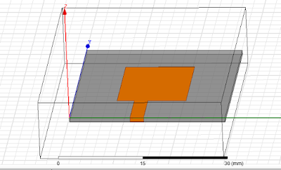
Simulation of Microstrip Patch Antenna using HFSS software with analysis of rectangular plot, polar plot and smith chart.

Microwave Engineering Lab (BTEC-606)

Experiment No: 2

AIM: Simulation of Microstrip Patch Antenna using HFSS software with analysis of rectangular plot, polar plot and smith chart.

SOFTWARE USED: ANSYS HFSS 15.0.3

THEORY:

Microstrip Patch Antenna: A patch antenna (also known as a rectangular microstrip antenna) is a type of radio antenna with a low profile (small height and width), which can be mounted on a flat surface. It consists of a flat rectangular sheet or "patch" of metal, mounted over a larger sheet of metal called a ground plane. In telecommunication, a microstrip antenna (also known as a printed antenna) usually means an antenna fabricated using microstrip techniques on a printed circuit board (PCB). They are mostly used at microwave frequencies. An individual microstrip antenna consists of a patch of metal foil of various shapes (a patch antenna) on the surface of a PCB, with a metal foil ground plane on the other side of the board. Most microstrip antennas consist of multiple patches in a two-dimensional array. The antenna is usually connected to the transmitter or receiver through foil microstrip transmission lines. Microstrip antennas have become very popular in recent decades due to their thin planar profile which can be incorporated into the surfaces of consumer products, aircraft and missiles, their ease of fabrication using circuit techniques, the ease of integrating the antenna on the same board with the rest of the circuit, and the possibility of adding active devices such as microwave integrated circuits to the antenna itself to make active antennas.

Procedure:

NOTE: Only after the completion of 1st experiment, you can start this 2nd experiment from following steps:

Here is the link of  1st Experiment.

1.      Select air- press F (Then select the face)

2.      Go to edit-select-By name

3.      Select air (select the faces except bottom face)

4.      Go to HFSS

5.      Boundaries-assign-radiation

6.      Name: Radiation  ok

7.      Save the file

8.      Go to analysis

9.      Add solution

10.  Solution frequency= 7.5 Ghz

11.  Adaptive solution

12.  Maximum number of passes: 20

13.  Maxm deltas= 0.02   ok

14.  Then analysis setup 1-right click-add frequency sweep

15.  Sweep type: fast

16.  Frequency setup

17.  Type: linear step

18.  Start: 5 Ghz

19.  Stop: 10 Ghz

20.  Step size: 0.1 Ghz

21.  untick the save field ok

RUN THE PROJECT:

1.      Result- create modal solution data report-rectangular plot

2.      Category: sparameter

3.      Function: db

4.      New report

5.      Close

FOR RADIATION PATTERN:

1.      Result – Create far fields Report - Radiation pattern

2.      Category: rE

3.      Quantity: rE total

4.      Function: dB

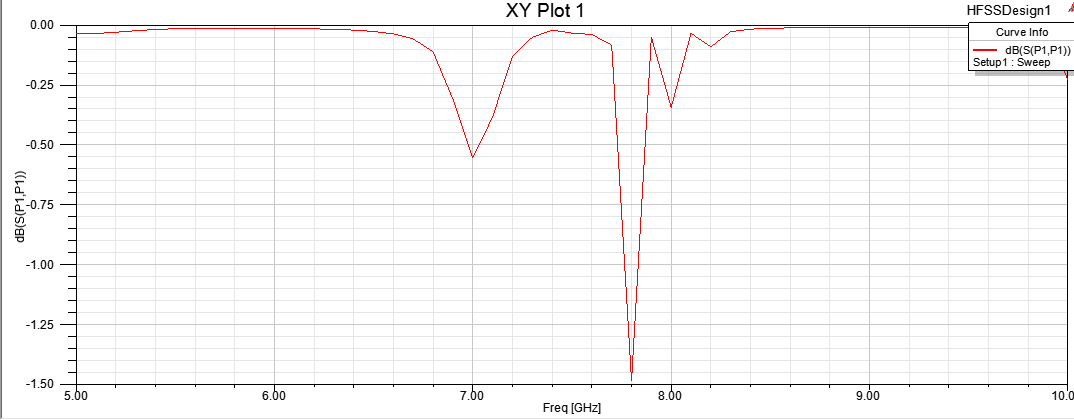
                                                                                                Figure: Rectangular plot

Figure: 3D polar plot

Figure: Smith chart